Use puq analyze to see all the available information stored in an HDF5 file after a UQ run. You can also use it to tweak PDFs, plot PDFs and response surfaces, or save them to files:
Usage: puq analyze [options] [hdf5_filename].
Type 'puq analyze -h' for option descriptions.

Options:
  -h, --help           show this help message and exit
  -v                   Verbose.
  --psamples=PSAMPLES  Filename CSV table of parameter samples.
  -r                   Re-analyze the data.
The - -psamples option is for use with externally generated samples for correlated input parameters. It is deprecated and may be removed in the future.
The -r option tells PUQ to reparse the output files and extract the data again before analysis. It is implied by - - filter. This option is not usually necessary.
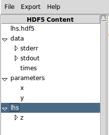
Here is a typical menu from puq analyze. Under data is the captured stdout and stderr for each job. The run times for each job is stored in times.
Under parameters is the list of input parameters.
All analysis, such as mean, deviation, sensitivity, response surface, and PDF, are stored in a section with the name of the method, followed by the output variable name. In the above example, it is “/lhs/z”.
If you are using a method that employs response surfaces, you can see (and sometimes tweak) it using puq analyze. What you see will differ depending on the response surface type. For example, Smolyak generates a best-fit polynomial response surface of the requested degree. MonteCarlo and LHS build a response function using Radial Basis Functions. By default it uses a multiquadric function, although you can change that.
Here are some examples from puq/examples/discontinuous/dome which is a very difficult surface to fit:
~/puq/examples/discontinuous/dome> puq start -f smolyak.hdf5 smolyak.py
Saving run to smolyak.hdf5

Processing <HDF5 dataset "z": shape (321,), type "<f8">
        Surface   = -10.1722431182861*x**6 - 31.8686981201172*x**5 + 47.3970642089844*x**4*y**2 -
        47.3970642089844*x**4*y + 130.954284667969*x**4 - 143.717315673828*x**3*y**2 +
        143.717315673828*x**3*y - 140.402770996094*x**3 + 113.759033203125*x**2*y**4 -
        227.51806640625*x**2*y**3 + 285.599304199219*x**2*y**2 - 171.840301513672*x**2*y +
        62.2936553955078*x**2 - 118.73616027832*x*y**4 + 237.472320556641*x*y**3 -
        197.646301269531*x*y**2 + 78.9101409912109*x*y - 11.4179744720459*x + 202.004089355469*y**6 -
        606.01220703125*y**5 + 703.17041015625*y**4 - 396.320373535156*y**3 + 111.905548095703*y**2 -
        14.7473888397217*y + 0.763792037963867
        RMSE      = 2.36e-01 (2.36e+01 %)

SENSITIVITY:
Var      u*            dev
-----------------------------
x    8.9079e-01    2.8561e+00
y    8.5187e-01    1.4274e+00
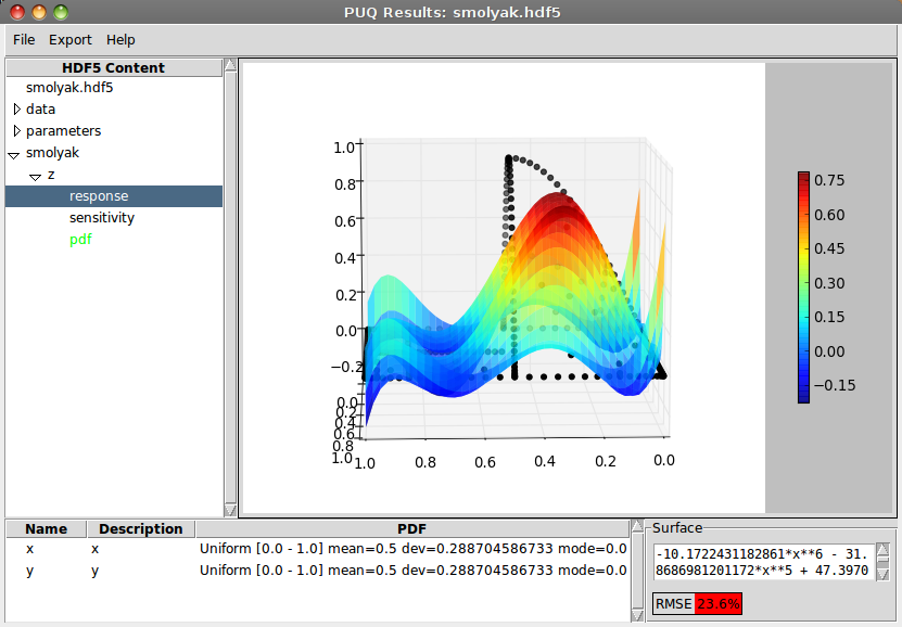
The sample points are in black. They are not on the response surface so you can see it is a poor fit. Notice also that the RMSE (Root Mean Square Error) is 23.6% which is high.
~/puq/examples/discontinuous/dome> puq start -f lhs.hdf5 lhs.py
Saving run to lhs.hdf5

Processing <HDF5 dataset "z": shape (500,), type "<f8">
Mean   = 0.211760030354
StdDev = 0.298137023113
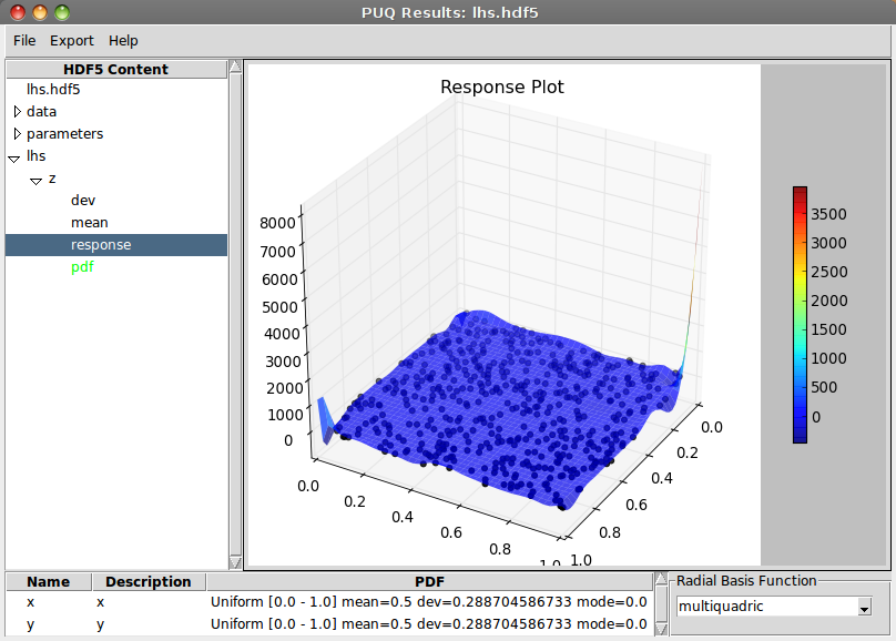
LHS with multiquadric RBF
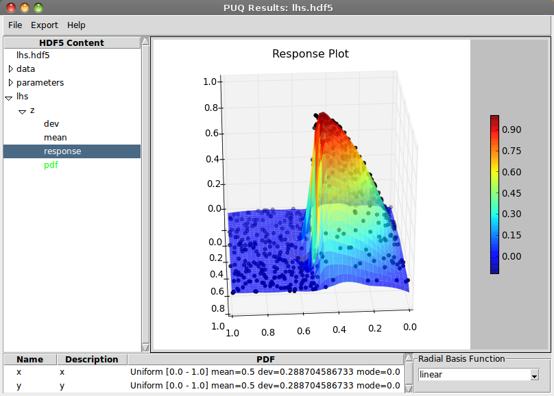
LHS with linear RBF
In the multiquadric fit, some spikes at the corners distort the response surface. A linear RBF appears to be the best fit.
PDFs will be listed in method/variable/pdf. If the word “pdf” is green, that indicates it is a placeholder for a PDF that will be calculated when you click on it. PDFs are calculated by sampling each input parameter (10000 times by default) and running those values through the response surface. The results are then displayed using a Kernel Density Estimate or a Linear fit. You can adjust those values as well as the minimum and maximum of the PDF. When you are finished adjusting the fit, the PDF can be saved as a plot or exported to the clipboard or a file. Exported PDFs can later be used as input parameters in other simulations or compared using puq read.