Monte Carlo Sampling

This is a simple example of using PUQ with a test program written in Python.

Rather than use a complex simulation as a test program, we will use the Rosenbrock function. This function is well understood and widely used as an example for optimization and UQ. Because it can be solved analytically, it is useful as a test case for our software.

The Rosenbrock function is \(f(x,y) = 100(y-x^2)^2 + (1-x)^2\)

And here is our python test program implementing it.

#!/usr/bin/env python

import optparse
from puqutil import dump_hdf5

usage = "usage: %prog --x x --y y"
parser = optparse.OptionParser(usage)
parser.add_option("--x", type=float)
parser.add_option("--y", type=float)
(options, args) = parser.parse_args()
x = options.x
y = options.y

z = 100*(y-x**2)**2 + (1-x)**2

dump_hdf5('z', z)

Most of the lines are concerned with parsing the command line. By default, PUQ expects test programs to take command line parameters in the format –varname=value. This is convenient for Python programs (using the optparse module) and C/C++ (using getopt). For existing test programs, you can easily instruct PUQ to pass parameters in another format. See Making PUQ Work With Your Code and puq/examples/matlab.

Line 16 calls dump_hdf5() with our output. dump_hdf5() takes three arguments, a name, a value, and an optional description. It formats the data so that PUQ can easily recognize it in standard output. It is placed in the HDF5 output file under ‘output/data/varname’ (‘output/data/z’ for our example). If we run our test program, we get:

~/puq/examples/rosen> ./rosen_prog.py --x=0 --y=1
HDF5:{'name': 'z', 'value': 101.0, 'desc': ''}:5FDH

So we have a working test program. We will limit x and y to [-2,2] and try to calculate an output PDF.

The next step is to write a control script to set up the sweep.

Here is what we will use

from puq import *

def run(num=20):
    # Declare our parameters here. Both are uniform on [-2, 2]
    p1 = UniformParameter('x', 'x', min=-2, max=2)
    p2 = UniformParameter('y', 'y', min=-2, max=2)

    # Create a host
    host = InteractiveHost()

    # Declare a UQ method.
    uq = MonteCarlo([p1, p2], num=num)

    # Our test program
    prog = TestProgram(exe='./rosen_prog.py --x=$x --y=$y',
        desc='Rosenbrock Function')

    return Sweep(uq, host, prog)

Every control script should look basically like this. There needs to be:

from puq import *

to import all the required PUQ code. There must be a function run() defined that returns a Sweep object. And the Sweep object is made up of a UQ method, a host, and a test program.

The UQ method is selected in the line:

uq = MonteCarlo([x,y], num=num)

This tells PUQ to use the Monte Carlo method, with two parameters ‘x’, and ‘y’. It will generate num random numbers each for ‘x’ and ‘y’, using a uniform distribution over [-2,2].

Now we are ready to run. We do this with ‘puq start rosen_mc’. Because control scripts are python scripts, the ‘.py’ is optional. Here are three runs, all doing 20 samples.

~/puq/examples/rosen> puq start rosen_mc
Saving run to sweep_52410436.hdf5

Processing <HDF5 dataset "z": shape (20,), type "<f8">
Mean   = 463.467551273
StdDev = 499.225504146

~/puq/examples/rosen> puq start rosen_mc 20
Saving run to sweep_52410475.hdf5

Processing <HDF5 dataset "z": shape (20,), type "<f8">
Mean   = 266.371029691
StdDev = 362.362400696

~/puq/examples/rosen> puq start -f mc.hdf5 rosen_mc 20
Saving run to mc.hdf5

Processing <HDF5 dataset "z": shape (20,), type "<f8">
Mean   = 322.364238869
StdDev = 246.016024931

As you can see, 20 samples is not enough to get an accurate mean. To get Monte Carlo Sampling to converge on a more accurate value, you would need to run thousands of samples. That is fine in a simple case like the Rosenbrock function, but a complex simulation might take days or weeks per sample.

To plot the response surface:

~/puq/examples/rosen> puq plot -r mc.hdf5

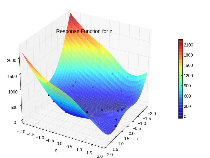
Scatter plot for Rosenbrock function using Monte Carlo with 20 samples.

Extending the Sample Size

In the example above, only 20 samples were used. If you wish to use more samples, you can modify your control script and rerun it from the start. However, if you do it this way, you are wasting the work that has already been done running the 20 jobs. That might be fine for a trivial example like this, but not for a complex simulation that ran for days to complete 20 jobs.

Fortunately you can easily add more samples to an existing Monte Carlo run:

~/puq/examples/rosen> puq extend --num 80 mc.hdf5
    Extending mc.hdf5 using MonteCarlo

    Processing <HDF5 dataset "z": shape (100,), type "<f8">
    Mean   = 377.988520682
    StdDev = 599.985509368

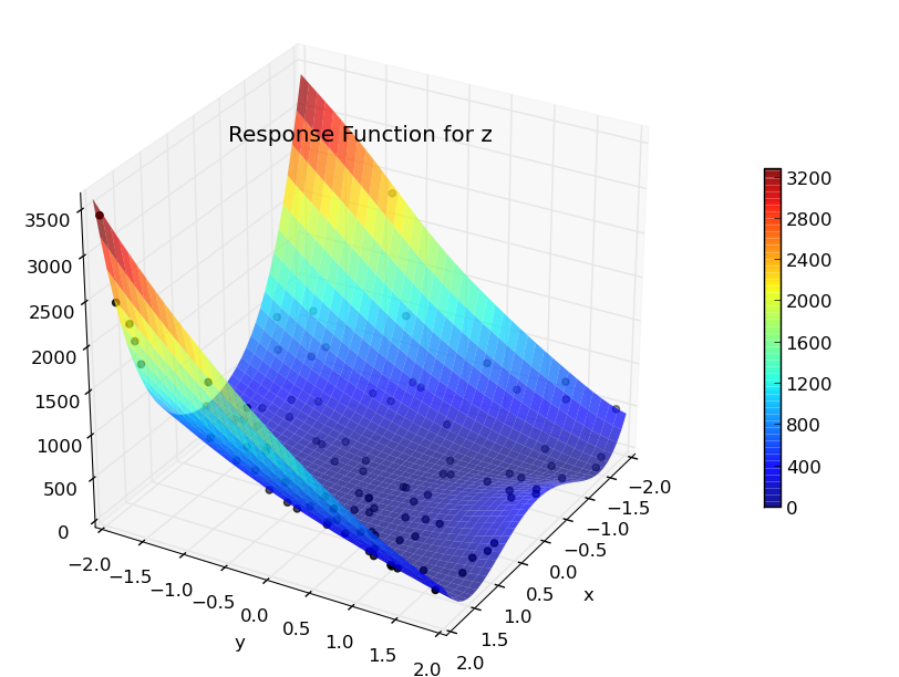
Scatter plot for Rosenbrock function using Monte Carlo with 100 samples.

The response surface now looks more accurate although the mean is still not close to the real mean. To plot the PDF of z, you can do:

~/puq/examples/rosen> puq plot mc.hdf5

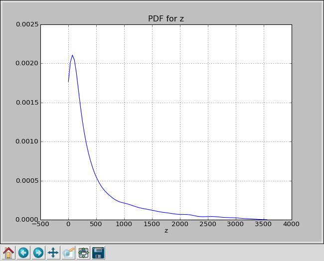
PDF for Rosenbrock function using Monte Carlo with 100 samples.