Note
The following information shows how to use the old ‘plot’ function. You may find it more convenient to use the plot function in analyze instead.
There are two main options for plotting:
By default, plots will be rendered to the current display. If you want the to plot to a file, use -f.
~> puq plot -h
Usage: puq plot [options] hdf5_filename.

Examples:
plot                  Plots all output PDFs. This is the default.
plot -k               Plots output PDFs using Gaussian Kernel Density.
plot -l -k            Plots output PDFs using Gaussian KDE and linear interpolation.
plot -v temp          If temp is an output variable, plots its PDF.
plot -v 'v1,v2'       Same as before, except plot v1 and v2.
plot -r               Plot response surface of output variables.
plot -r -v 'v1,v2'    Plots response surface of output variables v1 and v2.
plot -f fmt           Save plots. Valid values for 'fmt' are eps, pdf, png, ps, raw,
                      rgba, svg, and svgz.
plot -h               Help with additional options.

Options:
  -h, --help           show this help message and exit
  -r                   Response Surface Plot
  -v V                 Variable list. If multiple, put them in quotes and
                       separate by spaces or commas.
  -f F                 Format [pdf|ps|png|svg|i] [i]
  -l                   Plot output PDF using linear interpolation from a
                       histogram. [False]
  -k                   Use Gaussian Kernel Density Estimator on output PDFs.
                       [True]
  --nogrid             Don't show grid
  --title=TITLE        Title. Default is the Test Program description.
  --xlabel=XLABEL      Label for the X-axis. Overrides the default which
                       depends on the plot type.
  --ylabel=YLABEL      Label for the Y-axis. Overrides the default which
                       depends on the plot type.
  --zlabel=ZLABEL      Label for the Z-axis. Overrides the default which
                       depends on the plot type.
  --fontsize=FONTSIZE  Normal font size in points.
  --using=USING        Filename containing substitute parameter(s).
If your UQ run has more than one output variable, by default all of the output response surfaces or PDFs will be plotted. If you only wish to plot certain output variables, list them using the -v option.
When using -v, you don’t have to use quotes unless you have whitespace in your variable list.
In examples/basic, there are two input variables, ‘x’ and ‘y’ and three outputs, \(f(x,y) = x\), \(g(x,y) = y\), and \(h(x,y) = x + y\).
Run PUQ:
~/puq/examples/basic> puq start basic
Sweep id is 172906455

Processing <HDF5 dataset "f": shape (5,), type "<f8">
        Surface   = 1.0*x
        RMSE      = 0.00e+00 (0.00e+00 %)

SENSITIVITY:
Var      u*            dev
-----------------------------
x    1.0000e+01    0.0000e+00
y    0.0000e+00    0.0000e+00

Processing <HDF5 dataset "g": shape (5,), type "<f8">
        Surface   = 1.0*y
        RMSE      = 8.95e-12 (7.26e-11 %)

SENSITIVITY:
Var      u*            dev
-----------------------------
y    1.2317e+01    2.0001e-11
x    0.0000e+00    0.0000e+00

Processing <HDF5 dataset "h": shape (5,), type "<f8">
        Surface   = x + y
        RMSE      = 8.95e-12 (7.26e-11 %)

SENSITIVITY:
Var      u*            dev
-----------------------------
y    1.2317e+01    2.0002e-11
x    1.0000e+01    0.0000e+00
Note
The response of ‘f’ is ‘1.0*x’, the response of ‘g’ is ‘1.0*y’ and the response of ‘h’ is ‘x + y’. These are exactly as expected.
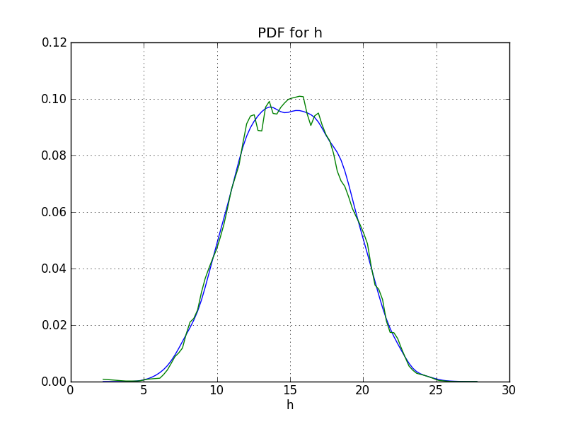
Plot the PDFs. Use the ‘l’ and ‘k’ flags to see both linear and Gaussian KDE fits:
~/puq/examples/basic> puq plot -lk -f png
plotting PDF for f
plotting PDF for g
plotting PDF for h
~/puq/examples/basic> ls -l *.png
-rw-rw-r--. 1 mmh mmh 28623 Jul  8 23:03 pdf-f.png
-rw-rw-r--. 1 mmh mmh 39468 Jul  8 23:03 pdf-g.png
-rw-rw-r--. 1 mmh mmh 40094 Jul  8 23:03 pdf-h.png
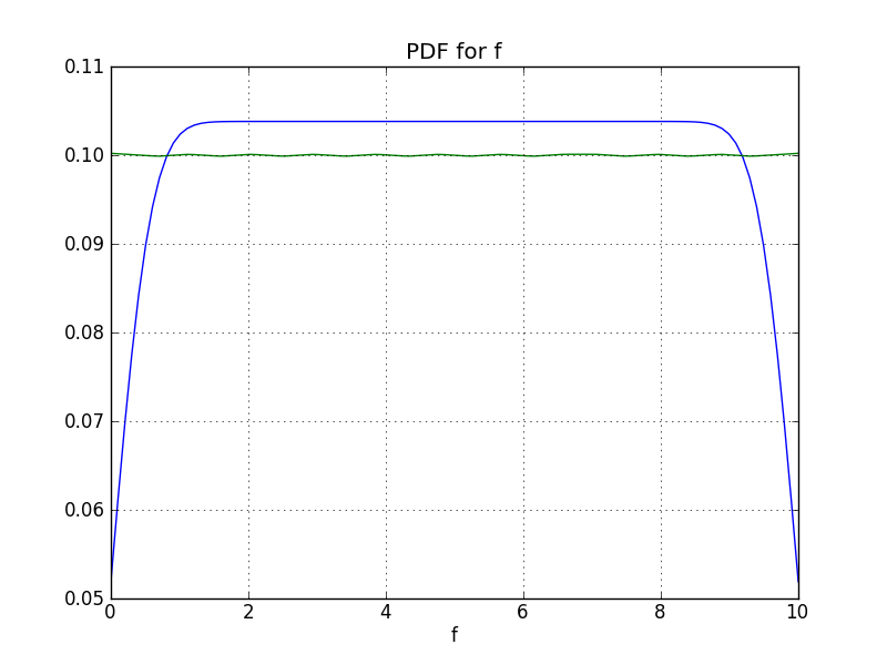
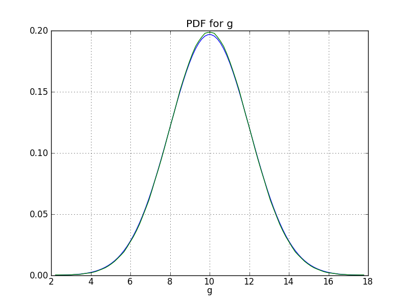
Click on an image to see it larger. You can see that the ‘f’ PDF is a Uniform distribution between 0 and 10. And the ‘g’ PDF is a Normal with a mean of 10 and deviation of 2. These are exactly as expected.