Modifying Smolyak Sweeps

Extending

If a Smolyak Sweep does not produce a good response surface, it is likely because the polynomial level was set too low. Fortunately we can easily extend a previous run, increasing its level by one. This is actually very efficient because each level uses all the information from the lower level. So some additional jobs will run and those results will be combined with all the previous results. For example:

~/puq/examples/rosen> puq extend sweep_140682290.hdf5
Extending sweep_140682290.hdf5 using Smolyak
Extending Smolyak to level 4

Processing <HDF5 dataset "z": shape (65,), type "<f8">
        Surface   = 100.0*x**4 - 200.0*x**2*y + 1.0*x**2 - 2.0*x + 100.0*y**2 + 1.0
        RMSE      = 3.96e-09 (1.10e-10 %)

SENSITIVITY:
Var      u*            dev
-----------------------------
x    5.0835e+03    6.9637e+03
y    1.9661e+03    1.7441e+03

Modifying Parameters & Reusing Response Surfaces

Sometimes after you run a simulation, you get new information that causes you to adjust your input parameters by a bit. Perhaps a new set of measurements allowed you to tighten up the deviation a bit. Or maybe the mean shifted some. If the input range has not widened significantly, the response surface should still be valid and you can use it with your updated input PDF(s). All PUQ has to do is sample the response surface with the updated PDF(s) to generate new output PDF(s).

For example, take a look at puq/examples/test1.

#!/usr/bin/env python
"""
Example of using a UQ method with a sweep.

Usage: test1.py
"""
from puq import *

def run():
    # Declare our parameters here
    v0 = Parameter('v', 'velocity', mean=10.0, dev=1.5)
    mass = Parameter('m', 'mass', mean=95, dev=8)

    # Which host to use
    host = InteractiveHost()
    #host = PBSHost(env='/scratch/prism/memosa/env.sh', cpus_per_node=8, walltime='2:00')

    # select a parameter sweep method
    # These control the parameters sent to the test program
    # Currently the choices include Smolyak, and PSweep
    # For Smolyak, first arg is a list of parameters and second is the level
    uq = Smolyak([v0, mass], 3)

    # If we create a TestProgram object, we can add a description
    # and the plots will use it.
    prog = TestProgram('./test1_prog.py', desc='Test Program One.')

    # Create a Sweep object
    return Sweep(uq, host, prog)

Run it to generate the response surface:

~/puq/examples/test1> puq start test1
Saving run to sweep_145215760.hdf5

Processing <HDF5 dataset "kinetic_energy": shape (29,), type "<f8">
        Surface   = 0.5*m*v**2
        RMSE      = 4.15e-08 (3.53e-10 %)

SENSITIVITY:
Var      u*            dev
-----------------------------
v    8.7761e+03    3.0974e+03
m    2.7263e+03    1.6263e+03
~/puq/examples/test1> mv sweep_145215760.hdf5 test1.hdf5

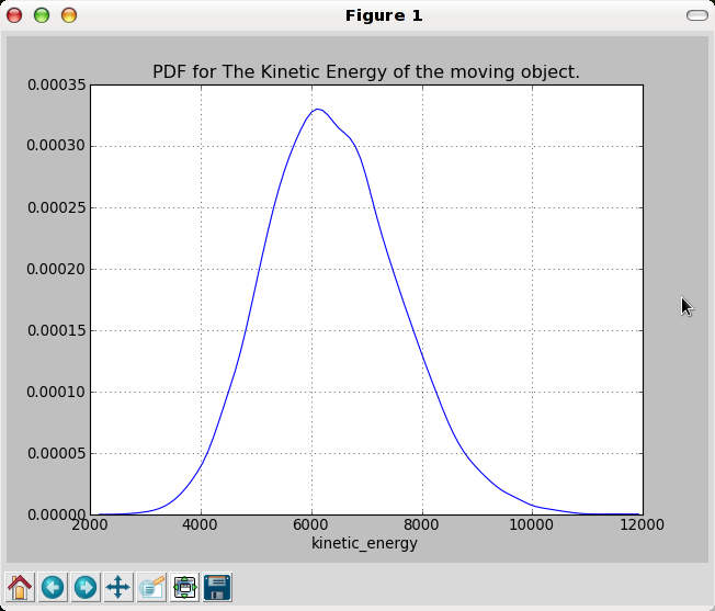
Later you want to recompute the output with new input PDFs. You will need to put the new Parameters in a file, with the same names (the first arg to Parameter). For example,

from puq import *

v = Parameter('v', 'velocity', mean=11.0, dev=1)
m = Parameter('m', 'mass', mean=105.0, dev=5)

Then you do ‘puq plot –using filename’:

/puq/examples/test1> puq plot --using new_pdfs.py  test1.hdf5
plotting PDF for kinetic_energy
REPLACING
        NormalParameter m (mass)
        PDF [63.9 - 126] 100 intervals
    mean=95  dev=7.99  mode=94.7
WITH
        NormalParameter m (mass)
        PDF [85.5 - 124] 100 intervals
    mean=105  dev=5  mode=105

REPLACING
        NormalParameter v (velocity)
        PDF [4.16 - 15.8] 100 intervals
    mean=10  dev=1.5  mode=9.94
WITH
        NormalParameter v (velocity)
        PDF [7.11 - 14.9] 100 intervals
    mean=11  dev=0.999  mode=11

test2.py is test1.py updated with the new parameters. You can do ‘puq start’ on it and compute a new response surface and PDF from scratch. It should match the one from test1 using the new parameters.

Note

PDFs are plotted by sampling the response surface with random numbers generated by the input PDFs. The resulting plot has some minor variances due to the randomness of the inputs.

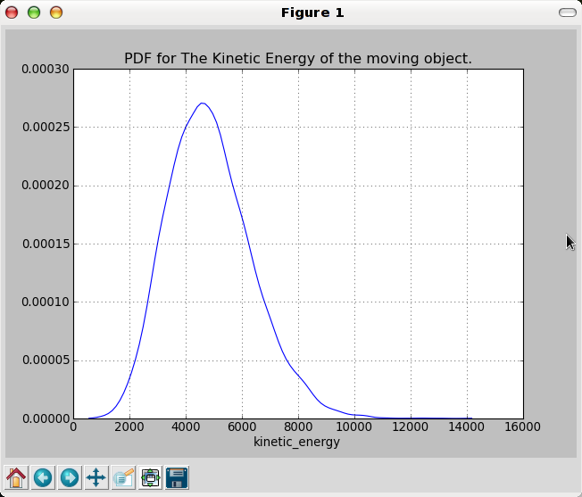
PDF from test1.py

PDF from test1 –using new_pdfs.py

PDF from test2.py.