In the last two sections, we have used Monte Carlo Sampling and Latin Hypercube Sampling on the Rosenbrock function. Both of those algorithms suffered from some common problems; they were slow to converge on a correct answer and their results were non-deterministic, varying from run to run due to the inherent randomness.
The Smolyak algorithm is a significant improvement. It uses a smaller number of runs to generate a response surface.
To move from Monte Carlo to Latin Hypercube sampling, we had to change a single line in our control script. To use Smolyak, we simply change that same line:
uq = LHS([x,y], num=num)
to:
uq = Smolyak([x,y], level=2)
Or use ‘rosen.py’ in puq/examples/rosen.:
~/puq/examples/rosen> puq start rosen
Saving run to sweep_140682290.hdf5

Processing <HDF5 dataset "z": shape (13,), type "<f8">
        Surface   = 301.0*x**2 - 2.0*x + 300.0*y**2 - 266.667*y - 345.667
        RMSE      = 7.40e+02 (2.05e+01 %)

SENSITIVITY:
Var      u*            dev
-----------------------------
x    3.9402e+03    5.2374e+03
y    2.0828e+03    1.8510e+03
The puq program first created a file using the unique id it generated. That file is sweep_140682290.hdf5. All information about this run is placed in there. The puq program next ran 13 jobs, using the parameters calculated by the Smolyak method. Then it calculated a response surface.
For the Smolyak method, the response surface should ge a perfect fit if the polynomial degree of the function is less than or equal to the Smolyak level parameter. For our example, we used a level 2 Smolyak run to approzimate a The Rosenbrock function, which is 4th degree. Because of this, the response surface does not exactly fit the data points. The RMSE is 20.5%.
PUQ also calculates the sensitivity of the parameters using the Elementary Effects Method
We can plot the response surface and pdf:
~/puq/examples/rosen> puq plot -r sweep_140682290.hdf5
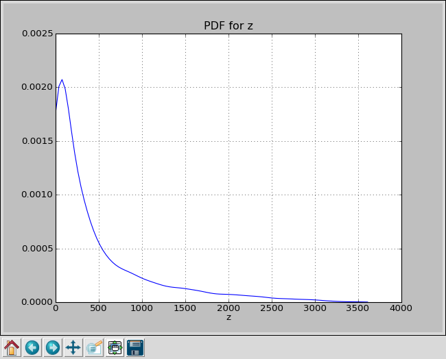
plotting PDF for z
And if you look at the response surface, you see the actual data as blue dots. Many of them are not on the response surface, indicating a bad fit.
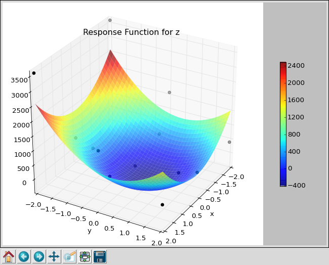
This is the output from a level-2 Smolyak, which required 13 jobs.
For comparison, here is the expected rosenbrock function.
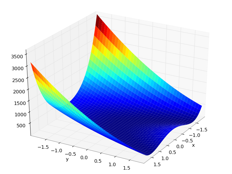
This is the rosenbrock function.
Next, if we bring up an editor and change the Smolyak level first to 3 then to 4, or do ‘puq extend’ twice, we get the following.
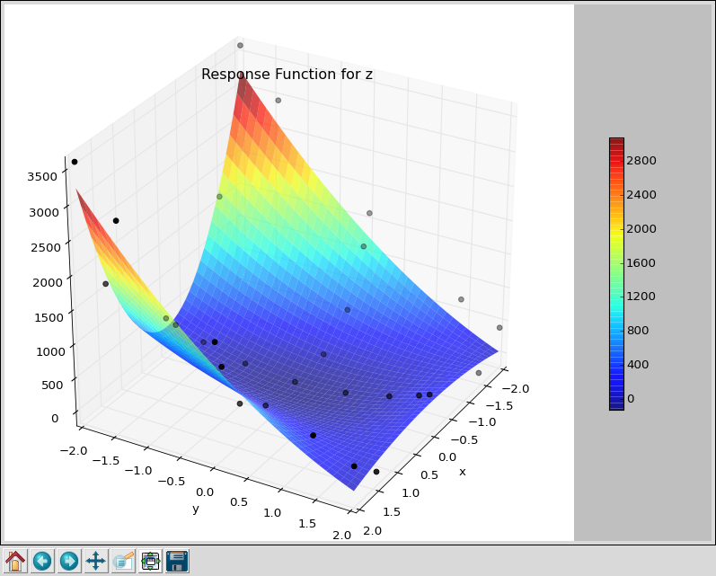
This is the output from a level-3 Smolyak, which required 29 jobs
 ~/puq/examples/rosen> puq extend sweep_140682290.hdf5
Extending sweep_140682290.hdf5 Using Smolyak
Extending Smolyak to level 3

Processing <HDF5 dataset "z": shape (29,), type "<f8">
        Surface   = -200.0*x**2*y + 343.857*x**2 - 2.0*x + 100.0*y**2 - 136.143
        RMSE      = 2.40e+02 (6.66e+00 %)

SENSITIVITY:
Var      u*            dev
-----------------------------
x    4.8307e+03    6.5106e+03
y    2.0022e+03    1.7623e+03
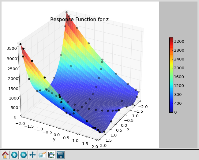
This is the output from a level-4 Smolyak, which required 65 jobs
~/puq/examples/rosen> puq extend sweep_140682290_A.hdf5
Extending sweep_140682290.hdf5 using Smolyak
Extending Smolyak to level 4

Processing <HDF5 dataset "z": shape (65,), type "<f8">
        Surface   = 100.0*x**4 - 200.0*x**2*y + 1.0*x**2 - 2.0*x + 100.0*y**2 + 1.0
        RMSE      = 3.96e-09 (1.10e-10 %)

SENSITIVITY:
Var      u*            dev
-----------------------------
x    5.0835e+03    6.9637e+03
y    1.9661e+03    1.7441e+03
PDF for Smolyak level 4, Rosenbrock function on [-2,2]
With 65 samples Smolyak outperforms Monte Carlo with 1000 samples.
Note
Smolyak is only suitable for cases where the response function can be approximated as a polynomial, at least over the input range with which we are concerned. For functions with abrupt changes or discontinuities, Latin Hypercube Sampling is probably a better choice.